G Code Viewer
Author: Connor
-
Boolean Algebra Circuits tool
Boolean_Algebra_Simulator Numerically Applied – Boolean_Algebra_Simulator
How it works: Select number of inputs (A–E). Add columns (layers) → add/edit/delete gates inside columns. Each gate wires to any previous-layer signal via dropdown. Gates in same column are parallel (no intra-column wiring). Select any signal as F. Truth table always evaluates correctly from gate types + connections. Expressions update on edit; use “Rebuild Expressions” after changing upstream gates. Final output shows both symbolic and traditional Boolean algebra form ( * = AND, + = OR, ! = NOT ).
Build your circuit, edit gates as needed, select output F, then Generate Truth Table.
-
Circuits 1 Calculator
circuits_equation_calculator.html Numerically Applied
circuits_equation_calculator.htmlEnter values in consistent SI units. Calculations auto-log to CSV (persisted in browser).
Basic Circuit Laws
1. Ohm’s Law — V = IR
Solves for any one variable when the other two are known. Fundamental starting equation.
2. Power in Resistor — P = VI / I²R / V²R
Computes power using any available pair. Derived from Ohm’s law substitutions.
Inductors & Capacitors — Basic Relations
3. Inductor Voltage — v = L di/dt
Voltage induced by changing current. Provide numeric di/dt at the instant of interest.
4. Capacitor Current — i = C dv/dt
Current due to changing voltage across capacitor.
5. Energy in Inductor — w_L = ½ L I²
Magnetic energy stored. Often used with i_L(0) initial condition.
6. Energy in Capacitor — w_C = ½ C V²
Electric energy stored. Dual of inductor energy.
First-Order RC & RL Circuits — Natural & Step Responses
7. RC Time Constant — τ = RC
Governs speed of exponential transients in RC circuits.
8. RL Time Constant — τ = L/R
Governs speed of exponential transients in RL circuits.
9. RC Natural Response — v(t) = V₀ e^(-t/τ)
Source-free capacitor voltage decay (t ≥ 0). Vss = 0. Find V₀ from DC analysis at t=0−. Matches source sheet algorithm.
10. RC Step Response — v(t) = Vss + (V₀ − Vss) e^(-t/τ)
Complete response when DC source is applied. Find Vss (t→∞, cap open) and V₀ (t=0−) first per PDF 5-step method.
11. RL Natural Response — i(t) = I₀ e^(-(R/L)t)
Source-free inductor current decay. I₀ from t=0− (inductor current continuous).
12. RL Step Response — i(t) = Iss + (I₀ − Iss) e^(-(R/L)t)
Complete response for RL circuit with DC source. Iss found with inductor as short-circuit (t→∞).
Second-Order RLC Circuits — Parameters & Transient Response Forms
13. RLC Parameters — α, ω₀, Damping Type, Roots / ωd
First step for any RLC analysis. Computes Neper frequency α and resonant frequency ω₀. Classifies overdamped / critically damped / underdamped and gives s1,s2 or ωd. Use exact formulas from source sheet step 5.
14. Overdamped RLC Response — r(t) = rss + A₁e^{s₁t} + A₂e^{s₂t}
For α > ω₀. Supply A1/A2 (solved from initial conditions i_L(0), v_C(0) per PDF) and s1/s2 from Parameters calculator. rss usually 0 for natural response.
15. Critically Damped RLC Response — r(t) = rss + (A₁ + A₂ t) e^{-α t}
For α = ω₀ (repeated root). Form includes linear t multiplier. Obtain α from Parameters calculator.
16. Underdamped RLC Response — r(t) = rss + e^{-αt} (A₁ cos(ωd t) + A₂ sin(ωd t))
For α < ω₀ (ringing case). Most common. Supply ωd and α from Parameters calculator. A1/A2 from initial conditions.
Calculation Log — CSV Data Store
Every successful calculation is automatically recorded here and saved in browser localStorage (persists across refreshes). Data is stored internally as a CSV structure. Use Export to download as .txt file (CSV content).
Timestamp Equation Inputs Result -

Common CNC Mill G-Codes: List
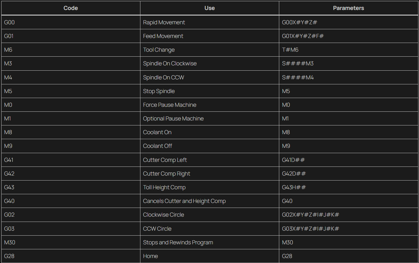
Code Use Parameters G00 Rapid Movement G00X#Y#Z# G01 Feed Movement G01X#Y#Z#F# M6 Tool Change T#M6 M3 Spindle On Clockwise S####M3 M4 Spindle On CCW S####M4 M5 Stop Spindle M5 M0 Force Pause Machine M0 M1 Optional Pause Machine M1 M8 Coolant On M8 M9 Coolant Off M9 G41 Cutter Comp Left G41D## G42 Cutter Comp Right G42D## G43 Toll Height Comp G43H## G40 Cancels Cutter and Height Comp G40 G02 Clockwise Circle G02X#Y#Z#I#J#K# G03 CCW Circle G03X#Y#Z#I#J#K# M30 Stops and Rewinds Program M30 G28 Home G28 G81 Straight Drill G81X#Y#Z#R#F# G82 Spot Drill G83X#Y#Z#R#P#F# G83 Peck Drill G83X#Y#Z#R#Q#P#F# G80 Stop Canned Cycle G80 G54-G59 Work offsets G54, G55, G56… G53 Cancels Work offsets and uses Machine Coordinates G53 Safety Codes
Code Use Parameters G17 Sets plane to XY Plane G17 G20 Set to Inches G20 G40 Cancels Height/Diameter Cutter Comp G40 G80 Cancels Canned Cycles G80 -
Circuit Analysis: Equation List
Basic Equations
Power Equations
Node Current
Mesh Current
Phasors
Transfer Functions
-
CNC Operator: GD&T
Basic Dimensions
Tolerances: Symetrical, Bilateral, Unilateral
Radius
UNLESS OTHERWISE SPECIFIED
Holes and Depths
Thread Tolerances
Datums
Feature Control Frame
General Precision
Datum Simulator
Selecting Pins
Calibration Stickers
-
Haas Machine: Operation
WCS
Offset Table
Height
WCS
MCSMemory Mode
Single Block
Op Stop
Edit Mode
MDI
Handle
-
Digital Logic
Section 1: Intro, Notation and basic operations
Boolean Algebra is very similar to regular algebra with a couple key differences. The only possible outputs are 1 or 0. 1+1+1… = 1.
As with regular algebra 1+0=1
Addition is equivalent to a Or Gate. The mathematic representation of a OR Gate, with Inputs A,B and Output C is.
Multiplication is equivalent to Multiplication. The mathematic representation of a AND Gate, with Inputs A,B and Output C is.
Multiple Gates can be added and multiplied. Two And Gates with Inputs (A,B), (C,D) and Output E is.
A NOT Gate is another fundamental component. The simplest explanation is it inverts whatever it is give 1=0 and 0=1. It will give the complement of whatever it is given. The representation of NOT A with Boolean Algebra is.
It is distributive
This can be built into equations. A NOR Gate is on as long as Both inputs are 0.
A NAND Gate is similar.
Demorgan’s theorem is a way to convert between AND and OR Gates. This will be a useful feature later.
Converting a NAND Gate to a OR gate is as follows. A NAND Gate is equivalent to Two NOT Inputs and a OR Gate.Converting a NOR Gate to a AND Gate is as follows. A NOR Gate is equivalent to Two NOT Inputs and a AND Gate.
Note: From this point further, i will be dropping the *, it would otherwise make the larger equations unnecessarily cumbersome.
XOR Gates
Section 2: Truth Tables
Truth tables provide every input and output, there are various useful things we can do with this, including create equations from truth tables.
A simple example for a AND Gate
A B C 0 0 0 0 1 0 1 0 0 1 1 1 This takes every possible input, and gives every possible output. Every Equation has a truth table and this can be used to convert equations and circuits into different gates. This is done occasionally for power efficiency, some types of gates are more efficient than others.
Section #: Minterm and Maxterms
You can derive various equations from a truth table. These equations are as a default in the MinTerm or Maxterm form. I will explain that in the next section
Section #: SR Latch
Section #: Karnaugh Maps
Karnaugh Maps are a type of Truth Table, which can be used to relatively easily simplify Equations into fewer Gates. In the given map, you draw various squares and rectangles in order to create various equations. With Karnaugh Maps, there are various rules and conventions for creating resulting equations/circuits.
Rules
- All selected outputs must be squares and rectangles.
- There must be a 2n number of ones, 2, 4, 8 are all valid while 3, 5, 6 and 7 are never valid.
- All cells must be horizontally or vertically, but not horizontally adjacent.
- There should be the fewest number of equations.
SAMPLE EQUATION
Truth Table
A B C D F Karnaugh Map
AB/CD 00 01 11 10 00 01 11 10 Section #: Finite State Machines
Or Gates
And Gates
D Latches
Multiplexers
Section 3: Circuit Design
Truth Tables
Time Graphs
Minterms and max terms
SOP AND POS
Karnaugh Maps
Don’t care
Half Adders
Full adders
Half Subtractor
Full Subtractor
Finite State Machines
-
Circuit Analysis
Section 1: Basic Circuit Analysis Groundwork
Name Symbol Use Units Amp A Current Flow A Columb C Electric Charge A · s Volt V Electric Potential kg · m² · s⁻³ · A⁻¹ Ohm Ω Resistance kg · m² · s⁻³ · A⁻² Watt W Power kg · m² · s⁻³ Joule J Energy kg · m² · s⁻² Farad F Capacitance kg⁻¹ · m⁻² · s⁴ · A² Henry H Inductance kg · m² · s⁻² · A⁻² Hertz Hz Frequency s⁻¹ Basic Equations
The Fundamental Equations we will use often throughout this course are.
V=IR is the simplest and most fundamental equation. Memorize it, we will be using it alot. Voltage(V) is Equal to Current(I) Multiplied by Resistance(R). You can rearrange this equation as needed. To solve for Current and Resistance.
Symbols
Section 2: Parallel and Series Calculations
The equation for Parallel Resistance is
The Equation for Series Resistance is
Exercise 1:
Section 3: KVL and KCL
Kirchhoff’s Voltage Law: All voltages in a Loop must add up to Zero.
EXAMPLE IMAGE
Kirchhoff’s Current Law: All Currents entering a node must add up to Zero
EXAMPLE IMAGE
Exercise 1: Solve for the Voltage in the Resistor R2
Exercise 2: Solve for the Current in Resistor R2
Voltage Drop
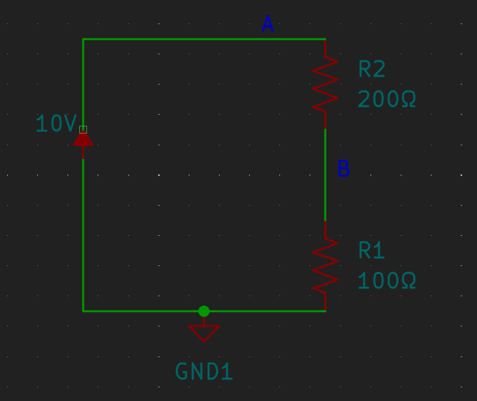
A necessary component of using KVL Effectively is Voltage Drop. Given two Resistors in Series, the Voltage drop across each of them will be proportional to the resistance. As a example, a 12v source, that runs through two resistors R1=1ohm and R2=2ohm. The Voltage Drop will be equal to.
This is true for any number of resistors in Series. The denominator represents Total Resistance in Series.
Rember this, it will be important later Voltage Division can be used to calculate the Voltage Drop across any Resistor. The Drop may not be relative to your ground(I will explain this with the Node Current method), but it will tell you the drop of the voltage across a resistor which can be used to calculate current.
Section 4: Power Equations
You can solve many equations using Conservation of Energy. Fundamentally this involved Power equations, the sum of all the power entering or leaving the system must be Zero.
The fundamental equations are.
Power is Equal to Current(I) times Voltage(V)
Power is equal to Current(I) Squared times Resistance
Power is equal to Voltage(V) Squared times Resistance
Exercise 1:
Section 5: Mesh Voltage and Node Current Methods
Two methods, that fundamentally are extensions of KVL/KCL are the Mesh Voltage and Node Current Methods. I will describe them together, then go into them separately. The Mesh Voltage and Node Current Methods, involve getting a series of Linear Equations, then solving them simultaneously. You can solve these linear equations manually, but i highly suggest using a calculator for this.
Mesh Voltage
Mesh Voltage fundamentally relies on Kirchoff’s Voltage Law, the Voltage in a Loop must equal Zero.
Node Current
Section 6: Source Conversion and Voltage Dividers
When evaluating a circuit, it may be convenient or necessary to convert between a voltage source and a Current source.
Section 7: Op Amps
Previously, before Digital Electronics Opamps were used to do analog Math operations.
Op Amps have a couple features and properties that make them very useful. Understanding these features and properties makes solving simple circuits with them extremely straight forward.
The Op Amp will try to make the Voltage of both Inputs equal. A Ideal Op Amp will not allow any current to pass through either input. The Voltage provided by the Output cannot exceed the Supply(+/-).
Features and Equations.
- Input(+)
Non-Inverting Input, Vin+
Must Equal Vin-
Vin- = Vin+ - Input(-)
Inverting Input, Vin-
Must Equal Vin+
Vin+ = Vin- - Vout
Output
Vout =A(Vin+ – Vin-) - Supply(+)
Provides power to the Op Amp
Vout Cannot exceed Supply(+) - Supply(-)
Provides power to the Op Amp
Vout Cannot exceed Supply(-)
Amplitude
Integrator Circuit
Sumer Circuit
Example 1:
Section 8: Applications of Calculus and Inductors/Capacitors
Capacitors and Inductors store energy in various ways. Capacitors store energy in Electric Potential, Inductors store Energy in a magnetic field. In DC circuits, when you apply a voltage and current to one of them, they eventually become Saturated.
The Natural Response, is when a Saturated Capacitor or Inductor is suddenly disconnected from the power source. What they do following that is called the Natural response, which is defined by First Order Differential Equations.
“n” here means for any quantity of resistors, capacitors or inductors that are all in either series of parallel.
Component: Resistance Capacitance Inductance Series: R1+R2+Rn=R 1/C1+1/C2+1/Cn=1/C L1+L2+Ln=L Parallel: 1/R1+1/R2+1/Rn=1/R C1+C2+Cn=C 1/L1+1/L2+1/Cn=1/L Equation R=V/I C=i(t)/(dv/dt) L=v(t)/(di/dt) Types of circuits RLC, RL, RC circuits
Natural response vs step response
There are various current equations for a Resistor, Inductor and Capacitor.
There are various voltage equations for a Resistor, Inductor and Capacitor.
RL First Order Differential Equation
RC First Order Differential Equation
RL Power EquationRC Power Equation
Time Constant
RC Example:
RL Example
From these we can get two differential equations which are straight forward to solve.
RC
RL
Section 9: Thevenin and Norton Equivalent Circuits.
Thevenin and Norton Equivalent circuits are ways to compress a more complicated circuit into a single equivalent Resistor and Voltage/Current Source. If you need to test various different components this can greatly simplify the system.
Thevenin Equivalent Steps
- Open the Load Resistor (Remove it from the circuit)
- Find the equivalent voltage for the given components Terminals
- Short all the Voltage Sources and Open all the Current Sources.
- Find the equivalent Resistance.
Example:
Norton Equivalent Steps
- Open the Load Resistor (Remove it from the circuit)
- Find the equivalent current for the given wire left by the Short.
- Short all the Voltage Sources and Open all the Current Sources.
- Find the equivalent Resistance.
Example:
Section #: AC Current
Sinusoidal Sources
VRMS
Steady Stage Response
Section #: Phasors
Capacitors and Inductors
Super Nodes and
Voltage and Current Source conversion
Thevenin’s Theorem
Thevenin Equivalent
OpAmps
Section 2: Capacitors, Inductors and Step Response
Section 3: AC Circuits and Phasors
Filter Circuits
Capacitors and Inductors
Response
- Input(+)
-
CNC Hand Programming
CNC Hand programming is handwriting programs. While as a fact no-one handwrites programs anymore, for beginners looking for in depth knowledge this is an extremely useful skillset.
This will be broken up in several sections. The first section is intended to be used as a reference for the Various codes. Don’t concern yourself with memorizing them, as you use them you will learn them very easily. There are less than 20 that you will commonly use.
G and M Codes: Numerical Control
To start, with some of the simplest and most basic codes, we have G01 and G00.
G00
G00 is for Bulk and Fast movement, do not use this for cutting. It is solely intended to move quickly from your current position closer to your material. Typically you will move to your X0.0 and Y0.0 then to a few inches above the part.Task: Move your tool to one inch above your part.
Example: (X0.0Y0.0 Center of Material) (Z0.0 Top of the Material) G00X0.0Y0.0; (moves to center of the part) G00Z1.0; (Moves to one inch above your part)G01
G01 is for cutting, you need a feed rate that is typically in Inches Per Minute (IPM). The Program will not run without a feedrate.Task: From your previous position, move to the bottom left corner, one inch away in the X and Y. Then move down and cut 0.020″ deep up to the top left corner one inch away in the X and Y. Use a Feedrate of Five Inches Per Minute.
Example: G01X-1.0Y-1.0F5.0; (Moves to bottom left corner) Z-0.010; (The Program will stay in G01 and reuse the feedrate of 5.0IPM) X-1.0Y1.0; (Moves directly up and travels two inches)M3 and M4
M3 will turn on your spindle Clockwise, M4 will turn your spindle on CounterClockWise. You will almost always use M3, nearly every CNC Machine tool is designed to turn Clockwise. S#### will set the speed in Rotations Per Minute (RPM). Be very careful that you did not mistype the speed value or it can severely damage something.Task: Turn the Spindle to 2500 RPM.
S2500M3; (Sets the spindle speed to 2500RPM, Then turns the spindle on Clockwise)Work Offsets: G54
Your work offset tells the Machine where your workpiece is. There is a separate Article about how to set your work offset here (LINK). For now we will assume it is already set.
For Mills, your Work Offset can be any number between G54-G59. It will include three numbers, your X, Y and Z values. Ensure these are set correctly, otherwise you can scrap a part or crash the machine.Task: Call your work offset.
Example: G54; (Sets your work offset to G54) (It is that simple, just don't forget it)Height Offsets: G43 and Height
Another set of Data you need to pay attention to is your Tool Height. All of your tools are different lengths, they can wear down, and when you replace them it’s nearly impossible to get them in the exact same place.G43 is the code to turn on height offset compensation. If you include a height offset value without it, the code will do nothing. Then you could scrap a part or crash the machine.
There is another Article on how to set your height. Your Height will be stored in your Tool Offsets, under the H#. # is whatever tool you are using. T5 is H5, when setting up, it is very common when setting up a machine to leave a tool in it’s existing position. When you do so make sure you change your Height Value as well.Task: Set your height value to H2
Example: G43H2;Tool Changes: M6
In order to run a program effectively you may need multiple tools, in order to toolchange, you use the code M6.Task: Switch to tool 19.
Example: T19M6; (Calls up T19 then switches tools with M6.)Exercise Section:
Create a program, that switches to T5, a half inch endmill. Then cuts a 1 inch square in the center of a 2 inch block using a spindle speed of 2,000 RPM and a Feedrate of 5IPM.Answer
O4001;
G90 G80 G40 G20 G17; (Safety line, explained in the next section)
T5M6; (Selects Tool 5 and switches using M6)
G43H5; (Enables Length based compensation with G43 and Selects Height 5)
G54: (Selects work offset G54)
(Rapid Moves)
G00X0.0Y0.0;(Moves to X0Y0)
<INCOMPLETE>Radial offsets: G41 and G42
Often, your tool will not be the exact right size for the task. It may be 0.001″ too big or “-0.003 too small. We can compensate for this using G41 and G42, this is often handled by the CAM Software, but here we will do this manually.
The Offset D number will have two numbers a Diameter which is typically set to 0.000, and a Wear offset. The Wear offset is used to make small adjustments. You can program you toolpath to match a specific tool, such as a 1/4″, 3/8″ or 1/2″, or more rarely you can program the toolpath to follow the edge of your part. Then set the Diameter to the size of your tool. This is uncommon and will typically only be done when learning. We will do it in the next exercise.G41: Offsets the Tool to the Left of the Toolpath.
G42: Offsets the Tool to the Right of the Toolpath.
If your tool is travelling on the near side of a block, left to right. You would use G42, this offsets the tool to the Right, which will compensate for your wear or tool size. If travelling from right to left, you would use G41. This offsets the tool to the left of the tool path.
Task:
Canned Cycles
Radial Compensation
Exercise, Facing program
Exercise 123 Block
Feeds and Speeds